In Chap. 1, we discussed the general features of QIIME 2. In Chap. 2, we first introduce some useful R functions (Sect. 2.1). Then, we introduce some useful R packages for microbiome data (Sect. 2.2). In Sect. 2.3, we illustrate some specifically designed R packages for microbiome data including the phyloseq and microbiome packages. In Sect. 2.4, we briefly describe three R packages for analysis of phylogenetics including ape, phytools, and castor. In Sects. 2.5 and 2.6, we introduce the BIOM format and the biomformat package and how to create a microbiome dataset for longitudinal data analysis. Finally, we summarize the main contents of this chapter in Sect. 2.7.
2.1 Some Useful R Functions
This section illustrates some useful R functions. Most microbiome data analyses in this book will use R software (R version 4.1.2; 2021-11-01). Some general R functions, R packages, and specifically designed R packages for microbiome data analysis are very useful. Let’s first briefly introduce these functions and packages before we move on to other chapters.
The famous Iris data were collected by Edgar Anderson in 1935 (Anderson 1935) and first used by Fisher in 1936 (Fisher 1936) to illustrate a taxonomic problem. The dataset measures the variables in centimeters of sepal length and width, and petal length and width, respectively, for 50 flowers from each of 3 Iris species (setosa, versicolor, and virginica). The dataframe iris has 150 cases (rows) and 5 variables (columns) named Sepal.Length, Sepal.Width, Petal.Length, Petal.Width, and Species. The Iris dataset is wrapped in R package.
In this section, we use the Iris dataset to illustrate some useful R functions. In Chap. 4 (Introduction to R, RStudio, and ggplot2) of our previous book on microbiome data analysis (Xia et al. 2018), we introduced some basic R functions for data import and export, including read.table(), read.delim(), read.csv(), read.csv2(), and write.table(). Some of them such as read.csv() are used very frequently across most chapters in this book. Here, we introduce additional basic R functions that could be useful in your data analysis.
2.1.1 Save Data into R Data Format
Writing R data into txt, csv, or Excel file formats facilitates data analysis using other software, such as Excel. However, all these file formats have their own data structures rather than reserve the original R data structures, such as vectors, matrices, and data frames as well as column data types (numeric, character, or factor). The data files will be automatically compressed after the data are saved into R data formats (e.g., .rda files); thus, one benefit of saving data into R data formats can substantially reduce the size of converted files.
2.1.1.1 Use SaveRDS() to Save Single R Object
2.1.1.2 Use Save() to Save Multiple R Objects
2.1.1.3 Use Save.Image() to Save Workspace Image
By default, save.image() stores the workspace to a file named .RData. We can also specify the file name for saving the work space, such as to save the work space as “myworkspace” using save.image(file = “myworkspace.RData”). Actually, you may notice that each time when you close R/RStudio, you are asked whether or not to save your workspace. If you click yes, then the next time when you start R, the saved workspace (with .RData) will be loaded.
2.1.2 Read Back Data from R Data Format Files
The saved R files can be read back to R workspace using either readRDS() or load() functions.
2.1.2.1 Use ReadRDS() to Read Back Single R Object
2.1.2.2 Use Load() to Read Back Multiple Objects from R File
2.1.3 Use Download.File() to Download File from Website
The R function download.file() can be used to download file from a website, such as a webpage, an R file, a tar.gz file, etc. The simplest syntax of this function is with two arguments: download.file(url, destfile). url is a character string (or longer vector) naming the URL of the file to be downloaded; destfile is a character string (or vector) with the name where the downloaded file is saved (path with a file name). For example, to directly download the QIIME 2 files: “feature-table.qza” from the following QIIME 2 website to R or RStudio, we call the download.file().
2.2 Some Useful R Packages for Microbiome Data
There are very useful and often used R packages. In this section, we introduce and illustrate some of them.
2.2.1 Readr
In this section, we use the famous Iris data to illustrate some useful R package. The package readr was developed by Hadley Wickham et al. (Wickham, Hester, and Francois 2018) for fast reading and writing delimited files or csv files (current version 1.4.0, March 2022). It contains the function write_delim(), write_csv(), and write_tsv() to easily export a data from R. We continue to use the Iris dataset to illustrate the readr package.
Depending on data format, we can choose the write_delim(), write_csv(), or write_tsv() to export a data table from R. Of which, the write_delim() function is a general function of writing data from R; write_csv() is used to write a comma (“,”) separated values; while write_tsv() is used to write a tab separated (“\t”) values. The simplified general syntax of these functions is given as follows:
The built-in R iris dataset has been exported to a tab-separated (sep = “\t”) file called iris.txt in the current working directory: setwd(“~/Documents/QIIME2R/Ch2_IntroductionToR”).
2.2.2 Ggpubr
The R package ggpubr written by Alboukadel Kassambara (alboukadel.kassambara@gmail.com) (Kassambara 2020-06-27), is a ggplot2-based package that provides some easy-to-use functions for creating and customizing publication ready plots (current version 0.4.0, March 2022). The ggplots package written by Hadley Wickham (2016) is an excellent and flexible visualization tool in R. However the default generated plots are not ready for publication. Furthermore, the customized ggplot syntax is opaque, which challenges the R beginners and researchers with no advanced R programming skills. The ggpubr package facilitates the creation of beautiful ggplot2-based graphs with some key features, including less opaque syntax than the wrapped ggplot2 package, providing publication-ready plots, is able to automatically add p-values and significance levels to box, bar, and line plots, facilitating arranging and annotating multiple plots on the same page, and changing graphical parameters (e.g., colors and labels). Here, we illustrate some plots that are useful for exploration of microbiome data.
2.2.2.1 Box Plots
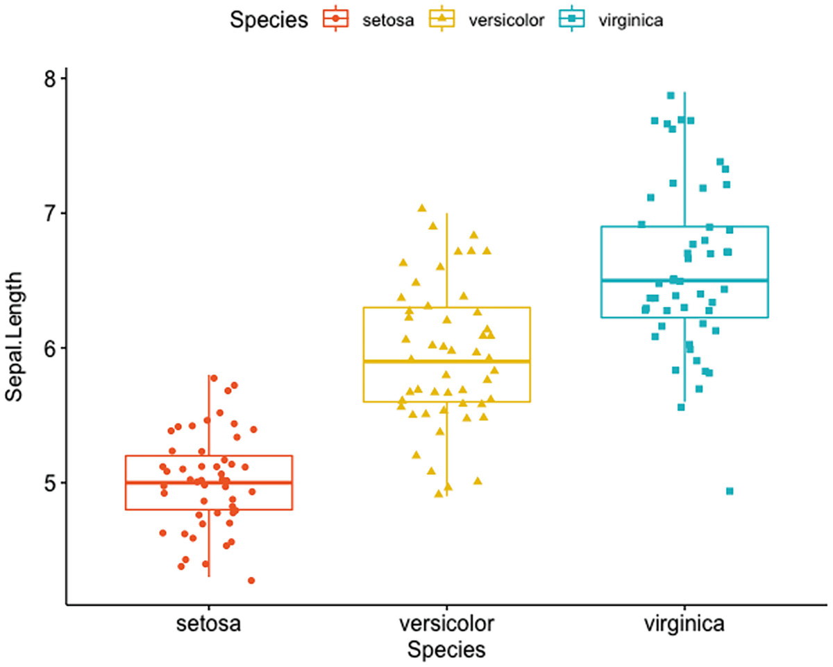
A box plot with jittered points has Sapel.Length versus species of setosa, Versicolor, and verginica. An Iris dataset of three species has different Sapel.Length, verginica has the highest and setosa has the lowest.
Box plots with jittered points using Iris dataset
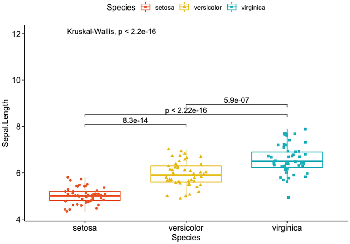
A box plot with jittered points has Sapel. Length versus species of Setosa, Versicolor, and Verginica. It depicts the p-value and p-values for pairwise comparisons of setosa versus versicolor, setosa versus virginica, and versicolor and virginica.
Box plots with a global p-value and p-values for pairwise comparisons
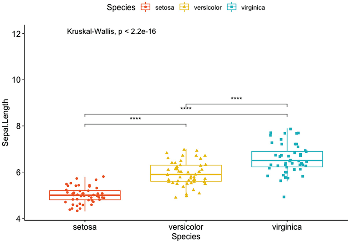
A box plot with jittered points has Sapel.Length versus species of Setosa, Versicolor, and Verginica. It depicts the p-value and the significance levels for pairwise comparisons of setosa versus versicolor, setosa versus virginica, and versicolor and virginica.
Box plots with a global p-value and the significance levels for pairwise comparisons
2.2.2.2 Violin Plots
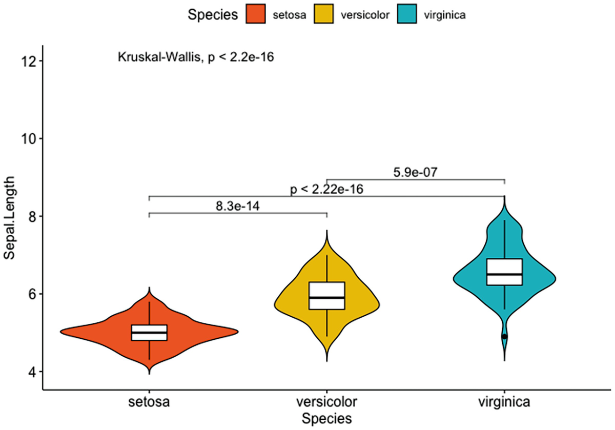
A violin plot with box plots has Sapel.Length versus species of setosa, versicolor, and verginica. It depicts that inside, adding the p-value and the p-values for pairwise comparisons of setosa versus versicolor, setosa versus virginica, and versicolor and virginica.
Violin plots with box plots inside adding a global p-value and p-values for pairwise comparisons

A violin plot with box plots has Sapel.Length versus species of setosa, versicolor, and verginica. It depicts that by adding the p-value and the significance levels for pairwise comparisons of setosa versus versicolor, setosa versus virginica, and versicolor and virginica.
Violin plots with box plots inside adding a global p-value and the significance levels for pairwise comparisons
2.2.2.3 Density Plots
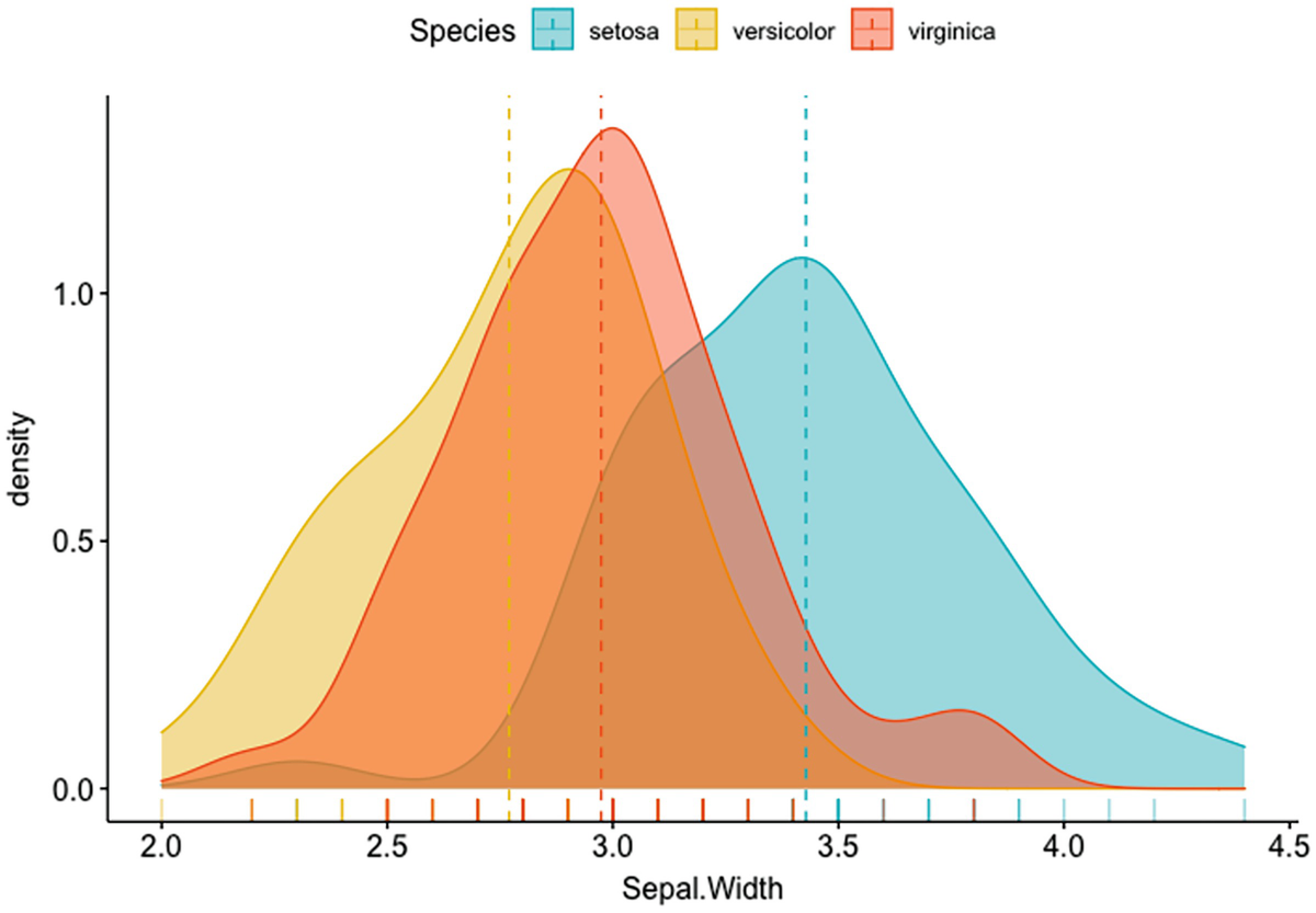
A plot depicts the density versus Sepal. Width with mean lines. It has a marginal rug that differentiates the colors of species.
Density plot of Sepal.Width with mean lines and marginal rug differentiating colors of species
2.2.2.4 Histogram Plots
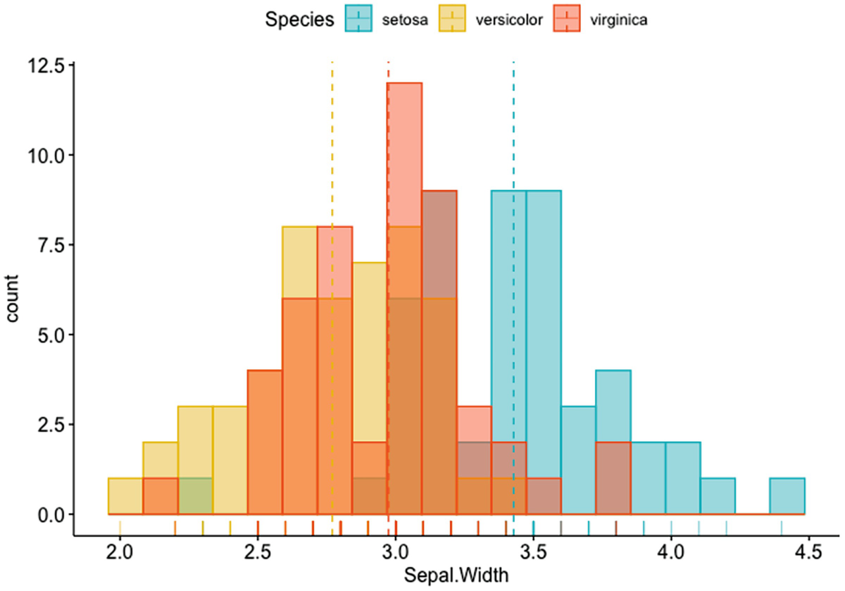
A histogram plot depicts the count versus Sepal. Width with mean lines. It has a marginal rug that differentiates the colors of species.
Histogram plot of Sepal.Width with mean lines and marginal rug differentiating colors of species
2.2.3 Tidyverse
The tidyverse package (a single “meta” package) was developed by Wickham et al. (Wickham et al. 2019) to collect R packages that share a high-level design philosophy and low-level grammar and data structures, enabling the R packages in the set work in harmony (current version 1.3.1, March 2022). The tidyverse is not the tools for statistical modelling or communication, instead its goal is to facilitate data import, tidying, manipulation, visualization, and programming. For example, it allows users to install all tidyverse packages with a single command. We can either install it from CRAN or via GitHub.
The tidyverse consists of four programs: (1) import, (2) tidy, (3) understand (transformation, visualize, and model), and (4) communicate. The programming works out this way (Wickham et al. 2019): starts with data import➔ tidy data➔ data transformation➔ understanding data: visualization and modelling➔ communication.
2.3 Specifically Designed R Packages for Microbiome Data
In this section, we introduce some specifically designed R packages for microbiome data analysis.
2.3.1 Phyloseq
The phyloseq package was developed to handle and analyze the high-throughput microbiome census data. The package was written by McMurdie and Holmes (McMurdie and Holmes 2013) with contributions from Gregory Jordan and Scott Chamberlain (McMurdie and Holmes 2022) (current version 1.36.0, March 2022). The phyloseq classes and tools facilitate the import, storage, analysis, and graphical display of microbiome census data. The phyloseq package mainly wraps statistical functions from vegan package (F. Jari Oksanen et al. 2018) and ggplot2 graphical package (Wickham 2016). Among the classes and tools, the phyloseq object and the operations on this object are very useful. The object and some functions of data operations have been adopted in other R microbiome packages for data processing and analysis such as in packages curatedMetagenomicData (Pasolli et al. 2017) and microbiome (Lahti 2017).
O’Keefe et al. in 2015 (S.J.D. O’Keefe et al. 2015) reported a 2-week diet swap study between western (USA) and traditional (rural Africa) diets to investigate whether the higher rates of colon cancer are associated with consumption of higher animal protein and fat, and lower fiber. The data is available for download from Data Dryad (S.J.D. O’Keefe 2016).
The dataset contains a HITChip data matrix and a sample metadata. The HITChip data matrix is a csv file which contains 222 samples from this study, providing the absolute HITChip phylogenetic microarray signal estimate for 130 taxa (genus-like groups). The sample metadata is also a CSV file, containing various measurement variables, in which SampleID is the unique sample identified corresponding to samples in the HITChip data matrix; subject is the subject identifier (some subjects have multiple time points); bmi is the standard body-mass classification (defining underweight, bmi <18.5; lean, 18.5≤bmi <25; overweight, 25≤bmi <30; obese, 30≤bmi <35; severe obese, 35≤bmi <40; morbid obese, 40≤bmi <45; superobese, bmi >45); sex (male/female); nationality is African American (AAM) and Native African (AFR); timepoint.total refers to the time point in the overall dataset ranging from 1 to 6; timepoint.group is the time point (1/2) within the group and group the sample treatment group representing Dietary intervention (DI)/Home environment (HE)/Solid stool pre-colonoscopy (ED).
2.3.1.1 Create a phyloseq Object
Microbiome abundance and taxonomic datasets are generated by next-generation sequencing (NGS) techniques. Currently 16S rRNA gene sequencing and whole-metagenome shotgun sequencing are the two most commonly used sequencing approaches (Xia and Sun 2022).
After taking initial quality control steps to account for errors in the sequencing process, the data generated by microbiome community sequencing typically are organized into large matrices where usually the columns represent samples, and the rows contain observed counts of clustered sequences commonly known as operational taxonomic units (OTUs/ASVs) that represent types of bacteria or other features. We often call these tables as OTU/ASVs tables or feature tables. We will introduce how to build feature table from raw sequencing reads in Chap. 4, assign taxonomy, building phylogenetic tree in Chap. 5, and cluster OTUs in Chap. 6. For now, we focus on how to create a phyloseq object in the phyloseq package.
One important concept and procedure in phyloseq package is the phyloseq object. A full phyloseq object has four data components: otu_table, sample_data, tax_table, and phylo. At least two components are needed to analyze the data of phyloseq object. The phyloseq object is created via the phyloseq() function. When the phyloseq object is created, the validity and coherency between data components is checked by the phyloseq-class constructor, which is invoked internally by the importers.
Step 1: Set the R working directory to the folder that these datasets are stored and load these datasets.
Step 2: Check and make sure that the datasets have been correctly loaded.
Step 3: Check and make sure that the classes of datasets are correct.
Since the above codes show that both otu_table and tax_table components are data frames, we need to convert them into matrices.
Step 4: Create phyloseq object using either phyloseq () or merge_phyloseq().
Now we can create a phyloseq object. We first use the phyloseq() function as below. It is important to make sure to specify whether taxa_are_rows = TRUE or FALSE based on the loaded otu matrix. Here, taxa_are_rows = FALSE.
The above created phyloseq object shows that OTU Table has 37 taxa and 222 samples, Sample Data has 222 samples by 7 sample variables, and Taxonomy Table has 37 taxa by 3 taxonomic ranks. One mistake that sometime happens is that the order or names of sample IDs in OTU Table and Sample Data are not exactly matched. We can use the sample_names() function to check.
Step 5: Create phyloseq object with adding a random phylogenetic tree component.
Now merge the tree data to the phyloseq object we already have by using the merge_phyloseq(), or use the phyloseq () to build it again from scratch. The results should be identical.
2.3.1.2 Merge Samples in a phyloseq Object
The phyloseq package supports two completely different categories of merging data objects: merging two data objects and merging data objects based upon a taxonomic or sample variable, i.e., merging the OTUs or samples in a phyloseq object. Merging OTU or sample indices based on variables in the data is useful to reduce noise or excess features in an analysis or graphic. It requires that the examples to be merged in a dataset are from the same environment and the OTUs to be merged are from the same taxonomic genera. The usual approach is to use a table-join, and hence the non-matching keys are omitted in the result, where keys are Sample IDs or Taxa IDs, respectively.
Here, we illustrate how to merge sample within a phyloseq object via the merge_samples() function. This function is a very useful tool to test an analysis effect by removing the individual effects between replicates or between samples from a particular explanatory variable. By performing the merge_samples() function, the abundance values of merged samples are summed.
First, remove empty samples, i.e., remove unobserved OTUs (sum 0 across all samples). In this case, all samples have sum of OTUs > 0, so the object physeq3a is identical to the object physeq3.
2.3.1.3 Merge Two phyloseq Objects
The new otutax object only has the OTU table and taxonomy table. When we compare the physeq3b with the original physeq3 object, they are confirmed being identical, where the physeq3b is the object that is built up by the original physeq3 object by using the function merge_phyloseq(). The arguments to the merge_phyloseq() are a mixture of multi-component (otutax) and single-component objects.
2.3.2 Microbiome
The microbiome package was developed by Leo Lahti et al. (Lahti 2017). The package utilizes phyloseq object and wraps some functions of vegan (Jari Oksanen et al. 2019) and phyloseq (McMurdie and Holmes 2013) packages with less obscure syntax (current version 1.14.0, March 2022). It also uses tools from a number of other R extensions, including ggplot2 (Wickham 2016), dplyr (Hadley Wickham et al. 2020), and tidyr (Wickham 2020). Here, we introduce some useful data processing functions in this package.
The microbiome package is built on the phyloseq objects and extends some functions of the phyloseq package in order to facilitate manipulation and processing microbiome datasets, including subsetting, aggregating, and filtering. To install microbiome package of Bioconductor development version in R, type the following R commands in R Console or RStudio Source editor panel.
2.3.2.1 Create a phyloseq Object
Caporaso et al. (2011)(Caporaso et al. 2011) published a study to compare the microbial communities from 25 environmental samples and three known “mock communities” – a total of 9 sample types – at a depth averaging 3.1 million reads per sample. This study demonstrated excellent consistency in taxonomic recovery and diversity patterns that were previously reported in many other published studies. It also demonstrated that 2000 Illumina single-end reads are sufficient to recapture the same relationships among samples that are observed with the full dataset.
These datasets have been used to illustrate the R programs in the other software including the phyloseq package. We store three data in the directory “~/Documents/QIIME2R/Ch2_IntroductionToR”: (1) “otu_table_GlobalPatterns.csv”, (2) “tax_table_GlobalPatterns.csv”, and (3) “metadata_GlobalPatterns.csv”.
The microbiome package has some very useful functions for processing microbiome data. We introduce them below.
2.3.2.2 Summarize the Contents of phyloseq Object
After performing the summarize_phyloseq() function, we obtain the information of the “physeq” object, including whether it is compositional, minimum, maximum, total, average, and median number of reads, sparsity, whether any OTU sum to 1, number of singletons, percent of OTUs that are singletons (i.e., exactly one read detected across all samples), and number of sample variables. In this case, we have 7 sample variables: X.SampleID, Primer, Final_Barcode, Barcode_truncated_plus_T, Barcode_full_length, SampleType, and Description.
2.3.2.3 Retrieve the Data Elements of phyloseq Object
The following functions in microbiome package facilitate this kind of processing and are very useful for downstream statistical analysis using the microbiome and other R packages, such as retrieving the data elements from phyloseq object.
Next, we use the tax_table() function to retrieve the taxonomy table.
Finally, we can melt the phyloseq data as a data frame table for easier plotting and downstream statistical analysis.
2.3.2.4 Operate on Taxa
In microbiome data processing, we sometimes want to merge the desired taxa into “Other” category. The function merge_taxa2() is used to place certain OTUs or other groups into an “other” category. One syntax is given: merge_taxa2(x, taxa = NULL, pattern = NULL, name = “Merged”). The merge_taxa2 () function differs from phyloseq::merge_taxa () lies its last two arguments: here, we can specify the name of the new merged group, and we can specify a common pattern in the name to merge. Here, we merge all Bacteroides groups into a single group named Bacteroides.
2.3.2.5 Aggregate Taxa to Higher Taxonomic Levels
One operation on taxa (aggregating taxa to higher taxonomic levels) is particularly useful. When the phylogenetic tree is missing, the aggregate_taxa () function can be used to aggregate taxa.
When the phylogenetic tree is available, we can use the functions merge_samples(), merge_taxa(), and tax_glom().
2.3.2.6 Operate on Sample
2.3.2.7 Operate on Metadata
2.3.2.8 Data Transformations
The microbiome package provides a wrapper for transformation of standard sample/OTU. One syntax is given: transform(x, transform = “identify”, target = “OTU”, shift = 0, scale = 1), where x is a phyloseq-class object; transform is used to specify the method of transformation to apply including “compositional” (i.e., relative abundance), “Z,” “log10,” “log10p,” “hellinger,” “identity,” “clr,” or any method from the vegan::decostand function. The target argument is used to specify whether the transformation applies for “sample” or “OTU,” but this option does not affect the log transformation. The shift argument is used to specify a constant to shift the baseline abundance (in transform = “shift”), and the scale is used to scale constant for the abundance values (in transform = “scale”).
Now we transform the absolute abundances to relative abundances. By applying the transformation of “compositional,” abundances are returned as relative abundances in [0, 1], i.e., convert to percentages by multiplying with a factor of 100.
Other common transformations are also available in the microbiome package including “Z” and “shift.”
2.3.2.9 Export phyloseq Data into CSV Files
2.3.2.10 Import CSV, Mothur, and BIOM Format Files into a phyloseq Object
2.3.3 ampvis2
The R package ampvis2 was developed by Andersen et al. to analyze and visualize 16S rRNA amplicon data (Andersen et al. 2018) (current version 2.7.17, March 2022). Like the phyloseq and microbiome packages, ampvis2 mainly wraps statistical functions from vegan package and ggplot2 graphical package. The attractiveness of ampvis2 is that its syntax of functions is very simple, and their plots such as ordination have very visualized effects. We will introduce ampvis2 to calculate alpha diversity (in Chap. 9), to calculate beta diversity, and to perform ordination plots (in Chap. 10).
2.3.4 curatedMetagenomicData
Shotgun metagenomic sequencing has provided amount of data for studying the taxonomic composition and functional potential of the human microbiome. However, various challenges prevent researchers from taking full advantage of these resources. The Bioconductor package curatedMetagenomicData (Pasolli et al. 2017) was developed to overcome these challenges and help the more shotgun data available publicly for using to perform hypothesis testing and meta-analysis (current version 3.0.10, March, 2022). The curatedMetagenomicData data package was developed for distribution through the Bioconductor (Huber et al. 2015) ExperimentHub platform. The database of curatedMetagenomicData so far provides thousands of uniformly processed and manually annotated human microbiome profiles (Pasolli et al. 2017), including bacterial, fungal, archaeal, and viral taxonomic abundances and gene marker presence and absence from MetaPhlAn2 (Truong et al. 2015), in addition to quantitative metabolic functional profiles and standardized metadata, including coverage and abundance of metabolic pathways and gene families abundance from HUMAnN2 (Abubucker et al. 2012). Metagenomic data with matched health and socio-demographic data are provided as Bioconductor ExpressionSet objects, with options for automatic conversion of taxonomic profiles to phyloseq or metagenomeSeq objects for microbiome-specific analyses. In this book, we will not implement this package; the interested readers are referred to (Lucas Schiffer and Waldron 2021).
2.4 Some R Packages for Analysis of Phylogenetics
Evolutionary analysis (analyses of phylogenetic trees) provides insights of phylogenetics and evolution that facilitate comparative biology and microbiome study. In this section, we introduce three phylogenetic R packages: ape, phytools, and castor. Each package provides various functions for writing, reading, plotting, and manipulating, and even inferring phylogenetic trees. However, we focus on phylogenetic tree generation, writing, and reading and provide simple tree plotting. For building phylogenetic tree in QIIME 2, the reader is referred to Chap. 5 (Sect. 5.2).
In Sect. 2.3.1.1, we have created a phyloseq object using Example 2.4 (Diet swap between rural and western populations). Here we continue to use this dataset to illustrate the analyses of phylogenetics.
2.4.1 Ape
The R package ape stands for Analyses of Phylogenetics and Evolution and is a modern and useful software for the study of biodiversity and evolution (Paradis and Schliep 2018)(current version 5.6.2, March 2022).
Step 1: Generate random rooted and unrooted trees.
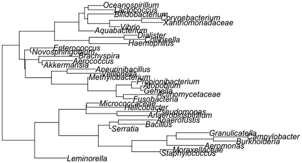
A schema of the phylogenetic tree depicts the topologies generated with equal frequencies, then the unbalanced topologies are generated in higher proportions than the balanced ones.
A random phylogenetic tree generated by the ape package using the Diet swap between rural and western populations
Step 2: Plot the random trees.
Step 3: Write the phylogenetic trees.
The generated tree can be easily written to and read back from files. The following commands write a rooted and an unrooted phylogenetic tree using the function write.tree():
Step 4: Read back the phylogenetic trees.
2.4.2 Phytools
Step 1: Generate random rooted and unrooted trees.
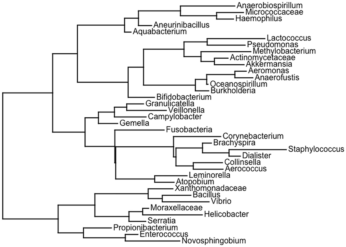
A schema of a rooted tree depicts phylogenetic comparative biology.
The rooted phylogenetic tree plotted by the plotTree () function via the phytools package using dietswap data
Step 2: Write the phylogenetic trees
The following commands write out this tree using the function writeNexus() from the phytools package.
This function writes a tree to file in Nexus format. It is redundant with ape::write.nexus(). The syntax is writeNexus(tree, “file = “”), where the argument tree is the object of class “phylo” or “multiPhylo”;
file is the file name for output.
Step 3: Read back the phylogenetic trees.
Step 4: Plot the phylogenetic trees.
2.4.3 Castor
The class “phylo” in phylogenetic tree is the most important data unit. It was introduced in ape in August 2002. The class “phylo” with the tree topology encoded in the member variable tree.edge. Most existing phylogenetic packages have been designed using the “phylo” format for much smaller trees containing at most a few thousand tips, and thus scale poorly to large datasets (Louca and Doebeli 2017). Unlike these existing phylogenetic packages, the R package castor (Louca and Doebeli 2017) was developed to compare phylogenetics on large phylogenetic trees (>10,000 tips)(current version 1.7.2, March, 2022). It provides efficient implementations of common phylogenetic functions, focusing on analysis of trait evolution on fixed trees. This package provides four kinds of functions: (1) efficient tree manipulation functions including pruning, rerooting, and calculation of most-recent common ancestors; (2) calculating distances from the tree root and pairwise distance matrices; (3) calculating phylogenetic signal and mean trait depth (trait conservatism); and (4) providing efficient ancestral state reconstruction and hidden character prediction of discrete characters on phylogenetic trees using maximum likelihood and maximum parsimony methods. Below we introduce how to write and read a tree in Newick (parenthetic) format using this package. For more information about Newick format, see Chap. 3 (Sect. 3.1.4).
Step 1: Write the phylogenetic trees.
The write_tree() function writes a phylogenetic tree to a file or a string, in Newick (parenthetic) format. If the tree is unrooted, it is first rooted internally at the first node. The syntax of this function is given:
The arguments: tree is a tree of class “phylo”; file is an optional path to a file, to which the tree should be written. The file may be overwritten without warning. If left empty (default), then a string is returned representing the Newick format tree; otherwise, the tree is directly written to the file. The argument append is a logical value that is used for specifying whether the tree should be appended at the end of the file, rather than replacing the entire file (if it exists). digits is an integer that is used to specify the number of significant digits for writing edge lengths; quoting is an integer, specifying whether and how to quote tip/node/edge names with 0, no quoting at all; 1, always use single quotes; 2, always use double quotes; −1, only quote when needed and prefer single quotes if possible; −2, only quote when needed and prefer double quotes if possible. The arguments include_edge_labels and include_edge_numbers are the logical values; they are used for specifying whether to include edge labels (if available) in the output tree, inside square brackets, edge numbers (if available) in the output tree, inside curly braces, respectively. These two arguments are an extension (Matsen et al. 2012) to the standard Newick format. This function write_tree() is comparable to (but typically much faster than) the ape function write.tree().
Step 2: Read back a tree from a string or file.
The read_tree() function loads a tree from a string or file in Newick (parenthetic) format. The syntax is given:
2.5 BIOM Format and Biomformat Package
The Biological Observation Matrix (BIOM) format(McDonald et al. 2012) or the BIOM file format (canonically pronounced biome) was designed to be a general-use format for representing biological sample by observation contingency tables (i.e., OTU tables, metagenome tables, or a set of genomes). BIOM is a recognized standard for the Earth Microbiome Project and is a Genomics Standards Consortium supported project. See more information on BIOM format in Chap. 3 (Sect. 3.1.3).
The biomformat package (McMurdie and Paulson 2021) is a utility package. Its use depends on other packages. It provides I/O functionality and functions to facilitate data processing from BIOM format files, such as providing tools to access data in “data.frame,” “matrix,” and “Matrix” classes.
Step 1: Read BIOM format file into R.
Step 2: Access BIOM data.
The biomformat package includes accessor functions. We can use them to access the data with BIOM format files.
The core “observation” data is stored in either sparse or dense matrices with the BIOM format. The sparse matrix support is carried with R via the Matrix package. We can use the biom_data() function to access the BIOM format matrices.
Obviously the accessed results from the fancier sparse Matrix of class are not easy to read. We can use the as() function to easily coerce the data to the simple, standard “matrix” class.
Observation metadata is metadata associated with the individual units being counted/recorded in a sample. For microbiome census data, it is often a taxonomic classification and something about a particular OTU/species. Here, the observations are counts of OTUs and the metadata is taxonomic classification, if present. In this case, the absence of observation metadata is reported. We can access observation metadata using the observation_metadata () function.
Sample metadata describe the properties of the samples. Similarly, we can access sample metadata using the sample_metadata() function.
Step 3: Write BIOM format data.
The following commands write the biom objects to a temporary file using the write_biom () function and then read it back using the read_biom () function and store it as variable infile. Next it checks whether these two objects are identical using the identical() function.
Step 4: Perform visualization and analysis on BIOM data.
2.6 Creating Analysis Microbiome Dataset
DiGiulio et al. (2015) conducted a longitudinal vaginal microbiome study to investigate the bacterial taxonomic composition for pregnant and postpartum women. This case-control study included 49 pregnant women, 15 of whom delivered preterm. The discovery data of 3767 specimens from 40 women were collected prospectively and weekly during gestation and monthly after delivery from the vagina, distal gut, saliva, and tooth/gum. The final dataset for pregnant women who delivered at term and preterm contained a total of 1271 taxa from 3432 specimens. Three datasets were downloaded and named as “TemporalSpatialOTU.csv,” “TemporalSpatialTaxonomy.csv,” and “TemporalSpatialClinicalMerged.csv,” respectively. The OTU data are available at species level. The taxonomy data are ranked at 7 levels: Kingdom, Phylum, Class, Order, Family, Genus, and Species. The available clinical information included race, weeks/days at the collection of samples, way of delivery, and household income level. The clinical data of 9 pregnant women in validated dataset is not available.
The study found that those women who with microbiome profiles had high abundances of Lactobacillus were less likely to experience preterm births, defined as delivery before gestational weeks. The study also found that those women who had high amounts of Prevotella had a higher occurrence of preterm births.
Step 1: Load raw microbiome datasets.
Step 2: Prune taxa using the gsub() function, and string pattern matching and replacement.
Step 3: Use the phyloseq and Tidyverse packages to filter and subset taxonomy and sample data.
Step 4: Use the Tidyverse and dplyr packages to finalize analysis dataset.
There are 64 sample variables in genus sample data. We can check the variable names using colnames(sample_data(genus)) or head(sample_data(genus)).
Finally, for ease of processing, we want to remove the variables that we do not use in the analysis. Although the tidyverse package contains the dplyr package, sometimes they are masked. In this case, we explicitly call the select() function of dplyr using the function dplyr::select().
Step 5: Use the Readr package to write the final analysis datasets to csv and tsv files.
For some readers, this example may be too complicated at the beginning chapter. Do not worry, you can skip these materials. When you read further in the later chapters, you can go back to look at these programs again; you will find that they are very useful.
2.7 Summary
Chapter 2 described and introduced some useful R functions, R packages, specifically designed R packages for microbiome data, and some R packages for analysis of phylogenetics, as well as BIOM format and biomformat package. The R programming language was created by statisticians Ross Ihaka and Robert Gentleman for statistical computing and graphics supported by the R Core Team and the R Foundation for Statistical Computing. R first appeared in August 1993 and the stable version 4.1.2 was released on November 1, 2021. R is available as open-source free software and is getting popular in academic research for statistical analysis and computing, and specifically is a main tool for development of statistical methods and models for microbiome and other omics studies. This chapter provided 6 sections on the R functions and packages for microbiome data analysis, including (1) useful R functions for saving, reading, and downloading data; (2) R utility and data visualization packages; (3) specifically designed R packages for microbiome data with focusing on the phyloseq and microbiome packages; (4) some R packages for analysis of phylogenetics; (5) BIOM format and biomformat package; and (6) creating analysis microbiome dataset. In Chap. 3, we will introduce some basic data processing operations in QIIME 2.